字数
1420 字
阅读时间
7 分钟
常用信号
[!note +] 函数
sawtooth三角波square方波sincsinc 函数之所以重要,是因为其 Fourier 变换正好是幅值为 1 的矩形脉冲。
锯齿波
octave
function [ output_args ] = example2_1( input_args )
clc;
clear;
fs=256;%采样频率
f1=50;
t=0:1/fs:1-1/fs;
y=sawtooth(2*pi*f1.*t);%乘以2pi表示出每秒变化的弧度数
plot(t,y);
xlabel('时间t/s');
ylabel('幅值');
end
下面的图分别为 f 1=30、50、70 


方波信号
octave
function [ output_args ] = example2_2( input_args )
clc;
clear;
fs=2048;%采样频率
f1=20;
t=0:1/fs:1-1/fs;
y=square(2*pi*f1.*t,0.5);
plot(t,y);
xlabel('时间t/s');
ylabel('幅值');
end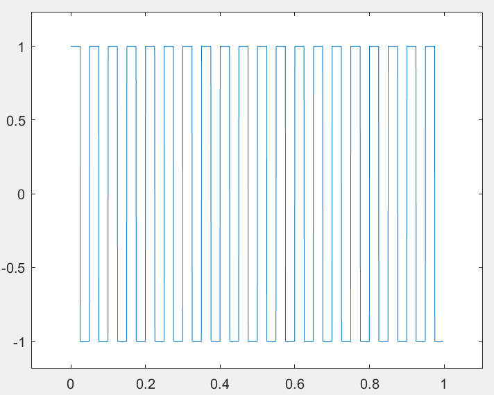 改变频率 w=50
 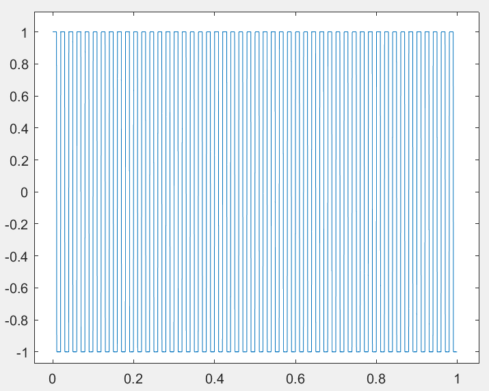 改变占空比为 80,频率仍为 30
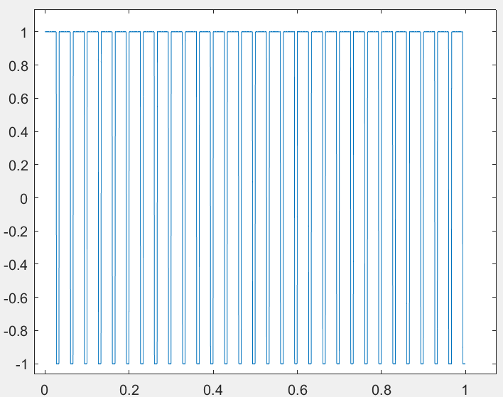
sinc 函数
octave
function [ output_args ] = example2_3( input_args )
clc;
clear;
t = linspace(-5,15);%这里默认是100
y = sinc(t);
plot(t,y);
xlabel('时间t/s');
ylabel('幅值');
end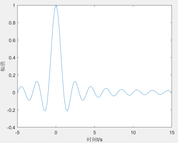 在这段程序里面,创建时间轴的过程中,
t = linspace(-5,15) 是默认在这一段区间分为 100 份,这个和 t= -5:0.2:15 类似,但有不同,前者是指定间隔数、后者是指定步长。 当我们将间隔数改为 50 时,可以发现下面的图就没有上面的图平滑。 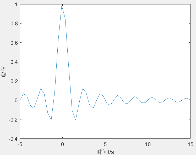
chirp 线性调频函数
octave
function [ output_args ] = example2_4( input_args )
clc;
clear;
fs=1500;%采样频率
f0=0;
f1=100;
t=0:1/fs:1-1/fs;
y=chirp(t,f0,1,f1);
plot(t,y);
xlabel('时间t/s');
ylabel('幅值');

end
发现后面的频率太高,绘制的时域图出现失真。 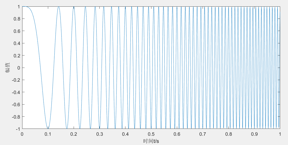
octave
function example2_4()
clc;
clear;
% 参数设置
fs = 1000;       % 采样频率
f0 = 0;          % 起始频率
f1 = 100;        % 终止频率
t = 0:1/fs:1-1/fs; % 时间向量
y = chirp(t, f0, 1, f1); % 生成线性调频信号

% 绘图
figure;
% 绘制时域信号
subplot(2, 1, 1); % 上图
plot(t, y);
xlabel('时间 t (s)');
ylabel('幅值');
title('线性调频信号');

% 绘制频谱图
subplot(2, 1, 2); % 下图
[~, f, ti, ps] = spectrogram(y, hamming(128), 120, 128, fs); % 计算短时傅里叶变换
surf(ti, f, 10*log10(ps), 'EdgeColor', 'none'); % 绘制时频图
axis tight;
view(2);
xlabel('时间 t (s)');
ylabel('频率 (Hz)');
title('线性调频信号的频谱图');
colorbar;
end
- 频谱图的代码解释
使用短时傅里叶变换 (STFT) 分析信号Ai(GPT-4o.)-短时傅里叶变换代码片段: matlab [~, f, ti, ps] = spectrogram(y, hamming(128), 120, 128, fs);
步骤和参数说明:
- 分帧:信号被分割成长度为 128 的帧,确保在每一帧内信号近似平稳。
- 窗口函数:
- 使用 Hamming 窗减少频谱泄漏。
- 帧移:帧间有 120 个采样点重叠,相邻帧之间存在 8 个采样点的间隔(128-120)。
- 傅里叶变换:对每一帧信号执行快速傅里叶变换 (FFT),得到该帧的频谱。
- 功率谱计算:
ps是功率谱密度,表示信号在不同时间和频率下的强度分布。
输出变量:
f:频率向量。ti:时间向量(表示每一帧的中心时间点)。ps:功率谱密度矩阵,行表示频率,列表示时间。
^e8d0ce
默认是线性调频 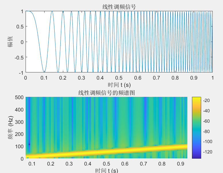
当频率调制的方法改为 quadratic 时,频率变化是二次的。 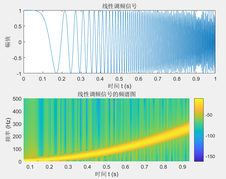
pulstran 重复冲击串
octave
function [ output_args ] = example2_5( input_args )
%EXAMPLE2_5 Summary of this function goes here
%   Detailed explanation goes here
clc;
clear;
% 定义时间向量 t,从0到10毫秒(10e-3秒),以20微秒(1/50e3秒)为步长
t = 0 : 1/50e3 : 10e-3;
% 创建延迟矩阵 d,其中第一列是脉冲出现的时间点,
% 第二列是每个脉冲的幅度衰减因子。这里使用了0.7的指数衰减。
d = [0 : 2/1e3 : 10e-3 ; 0.7.^(0:5)]';
% 使用 pulstran 函数生成一个由高斯脉冲组成的信号 y。
% 参数 @gauspuls 指定了脉冲的形状为高斯型,
% 10e3 是载波频率(10 kHz),0.3 是高斯脉冲的带宽因子。
y = pulstran(t, d, @gauspuls, 10e3, 0.3);
plot(t,y);
xlabel('时间t/s');
ylabel('幅值');
end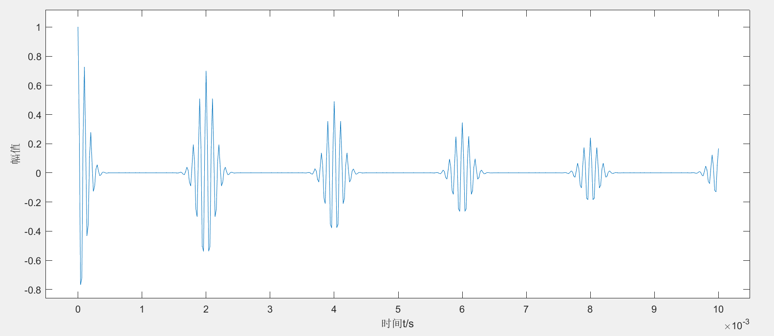
产生方波脉冲(非周期)
octave
function [ output_args ] = example2_6( input_args )
%EXAMPLE2_6 Summary of this function goes here
% Detailed explanation goes here
clc;
clear;
fs=1000;%采样频率
t=-1:1/fs:1;
y= rectpuls(t,0.6);
plot(t,y);
xlabel('时间t/s');
ylabel('幅值');
end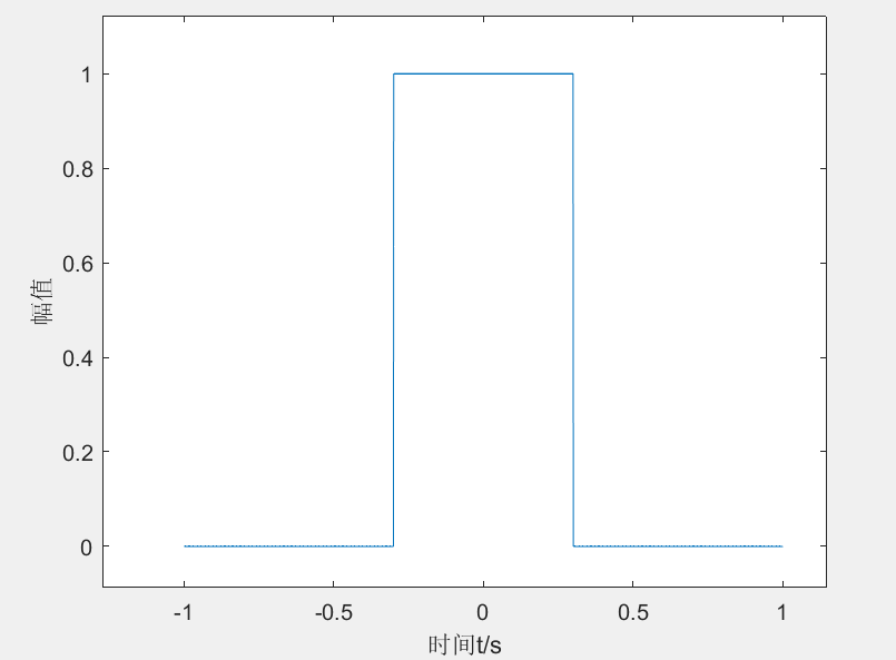 也可以在指定位置,加上指定脉冲宽度的矩形脉冲
octave
% 定义时间向量
t = -0.1:0.001:0.4;

% 定义脉冲位置和宽度
pulse_positions = [0, 0.2, 0.35]; % 脉冲开始的时间点
pulse_widths = [0.05, 0.07, 0.04]; % 对应的脉冲宽度

% 初始化信号为零
signal = zeros(size(t));

% 生成多个非周期矩形脉冲
for i = 1:length(pulse_positions)
    signal = signal + rectpuls(t - pulse_positions(i), pulse_widths(i));
end

% 绘制结果
figure;
plot(t, signal);
xlabel('时间 (秒)');
ylabel('幅值');
title('非周期矩形波');
grid on;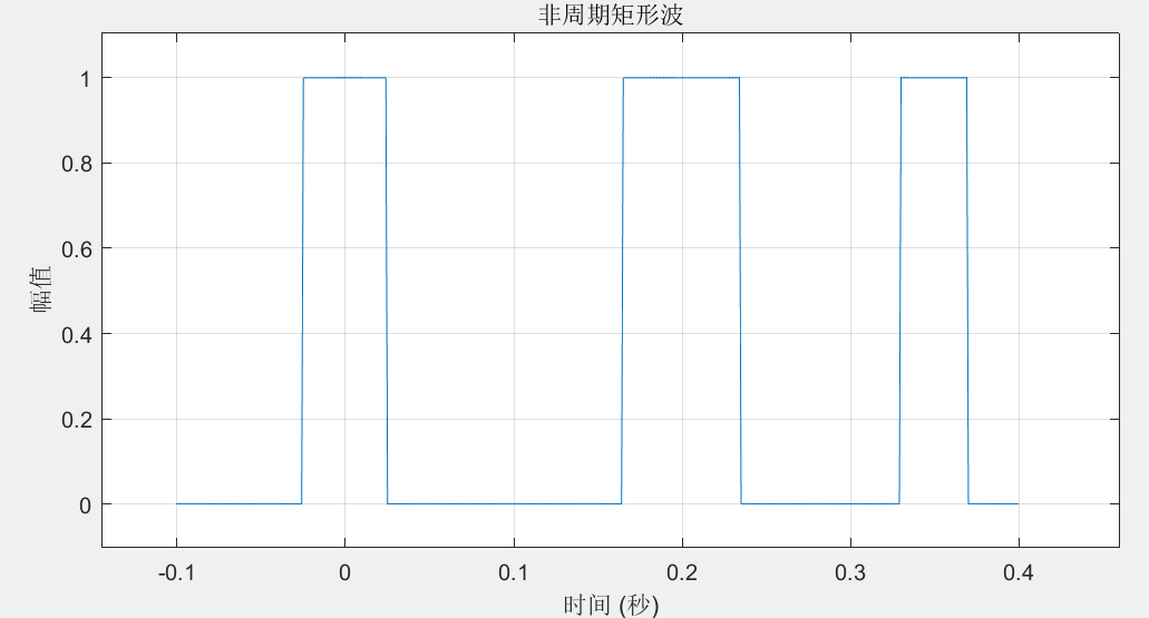
产生三角波脉冲(非周期)
octave
function [ output_args ] = example2_7( input_args )
%EXAMPLE2_7 Summary of this function goes here
%   Detailed explanation goes here
clc;
clear;
fs=1000;%采样频率
t=-1:1/fs:1;
y= tripuls(t,0.5);
plot(t,y);
xlabel('时间t/s');
ylabel('幅值');
end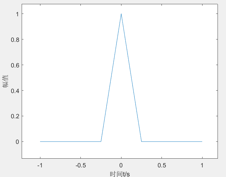
产生 Dirichlet 函数
什么是 [[AI(tongyi)-Dirichlet函数|Dirichlet函数]]
octave
function [ output_args ] = example2_8( input_args )
clc;
clear;
fs=1000;%采样频率
t=-1:1/fs:1;
% 使用 diric 函数计算 Dirichlet 函数值
% diric(t,N) 计算的是 N 周期的 Dirichlet 函数
% 这里使用了1000作为参数N,意味着函数在区间[-1, 1]内有1000个周期
y = diric(t, 1000);
plot(t,y);
xlabel('时间t/s');
ylabel('幅值');
end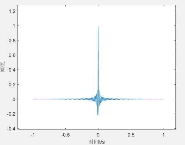
贡献者
 OveDuke